Get a callback from our team within 20 minutes during business hours.
Using the IF function in Excel can be very useful in a spreadsheet. The IF function will allow you to check if a condition you have set is true or false. You can use the IF function in a formula to give a result, depending on whether the data expressed in a cell meets the criteria.
For example, you could use the IF function in a spreadsheet of sales results and set the condition that if a salesman reaches a certain target, they will get a bonus. The IF function formula for the sales spreadsheet will look like this,=IF(A1>50000,”Bonus”,”No”)
There are three parts of the IF function, the logical test, the value if true and the value if false, so the basic IF function will look like this, =IF(logical_test,value_if_true,value_if_false,)
The logical test is the argument that you want the test for, is the number in the cell A1, greater than 50,000. For our example we use the (>) Greater than conditional operator.The ”Bonus” is if the value is true and “No” is if the value is false.
This is a basic IF function formula, but you can use other conditional operators in the formula.
< Less than
>= Greater than or equal to
<= Less than or equal to
<> Not equal to
In more complex IF function formulas, you are able to use a combination of these conditional operators.
Making a graph in a Excel spreadsheet is fairly simple and can be used to show data in a more visual format. There are different types of graphs available including, column, bar, line and pie charts. The type of graph that you use in a spreadsheet depends on the type of data results you need to show, as some graphs represent different results better than others.
Whatever style of graph you use, setting them up is all the same, in fact you can change you can switch between one style of chart to another and then just alter the layout of the graph to make it easier to read.
To start to create graph in Excel you need to enter the required data into a spreadsheet. You must remember to give your data in the spreadsheet labels.
Now click on the Insert tab on the Excel ribbon and then on have the charts panel that will present you with a selection of different graph types.
Once you have selected a type of graph, click on the select data tab. When the dialogue box opens you can either enter the cell range in the area, or click and drag the required cell area on the spreadsheet.
After you have created a basic graph, you can start to alter the design and look of it to what you require. Once a graph is created, it is easy to change from one style of graph to another.
If you click on the graph the chart tools group appears on the ribbon. On the design tab you can choose the layout for the chart. You can choose if you want your graph to have a title, the positioning of the axis titles and whether you want to show the graph legend. The design button will also allow you to switch the axis around.
The layout tab lets you edit the labels on your graph, including title and axis titles. It will also allow you to display the data labels on the graph, it will give you options to display the data as a percentage if you want.
By using the format tab, or right-clicking on the graph you can change the look of the chart, changing the colours of the data area, the plot and background areas and also the colour and size of the font used.
Sometimes when you are using Excel spreadsheets, you may find that you need to check cells for duplicate values, for example if you have merged data from two worksheets into one and you have to check if data has been duplicated. There are various ways of finding the duplicate values in content, but the simplest way to do this can be done using the Conditional Formatting button on the Home tab.
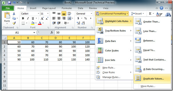
Select the columns and rows that you need to check for duplicates. You can click individual columns or rows, or you can hold down the Ctrl button and then select them. Then click on the Home tab and then the Conditional Formatting button to bring up the options box.
From the Conditional Formatting options box, click on the Highlight Cells Rules option and then select Duplicate Values.
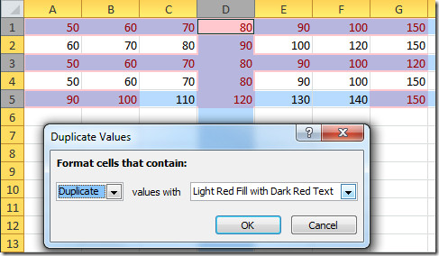
In the Duplicate Values dialogue box you can use the drop down menu to to choose how you want the duplicated values highlighted. Use the drop down menu to select the colour of the cell and the text and then click OK to finish.
Unique Values
You can also use the conditional formatting button to highlight Unique Values in a spreadsheet. Follow the same procedure as above then when you are in the Duplicate Values dialogue box, click on Unique in the drop down menu. This will now highlight the Unique Values in the spreadsheet.
One advantage of saving an Excel spreadsheet as a PDF file is that it allows someone to view the spreadsheet without owning the Microsoft Excel program. All they would need to view the PDF file is a PDF reader, such as Adobe Acrobat which is available for free download. Please note, you will only be able to view the Excel file in a PDF reader, but not change it in anyway. When you save a spreadsheet as a PDF you are given the option of saving particular sheets in a workbook, or the whole workbook itself.
In Excel, click on the file button and open up the spreadsheet or workbook that you want to save as a PDF file.
With the spreadsheet open, click on the file button again and when the options appear, click on the Save as button to open up the Save as dialogue box.
Choose a name for your PDF file.
Click on the arrow at the end of the Save as Type menu to bring up a list of file options and then click on PDF and then click Save.
Once you have clicked on Save, an Option button will appear in the Save as dialogue box.
Once you click on this Options button a new dialogue box will open up and this will allow you to choose what parts of the spreadsheet you wish to save. The default option is that all the pages of the current active spreadsheet will be saved.
In the Options dialogue box, you can check the Entire workbook option, or check the Selections options that will allow you to select what sheets of the workbook you want to save.
When you are finished with your options, click OK to close the dialogue box and then click Save to finish.
Your chosen spreadsheets or workbook will now be viewable in a PDF reader and can be shared with people who do not have access to the Excel program.
If you find that you have a lot of data to enter on your spreadsheet, it may be a good idea to create a drop down list to allow your users to enter data more easily. Having a drop down list will allow you choose from a set number of entries, so saving time. The cell that features the list will have a small arrow that when clicked will bring up the data options.
Create your list by in a column of cells, for example A1:A4. You are not restricted to entering the data in columns, you can also enter your list in a row, such as A1:D1.
Select the cell where you want to place your list. You can place the list in multiple cells if you need to.
Click the Data tab & then click the Data Validation button to bring up the dialogue box.
From the Allow options drop down list, choose List.
Click the Source box and select the cell range that contains the data that will make up your list. Alternatively you can enter the cell range manually, =$A$1:$A$4.
Make sure that you check both the in-cell drop down and the ignore blank boxes. The ignore blank box will allow users to make a blank selection.
While you are in the Data Validation box you can choose to set up an Input Message, such as Please Select and an Error Alert if the user tries to enter invalid data into the cell.
Click OK to finish.
If you wish to create a drop down list that is not dependent on data entered in other cells, you can enter the list items directly into the Source area in the Data Validation box and then continue with the rest of the above steps.
If you wish to delete the list from the worksheet, click on the cell to make it active and then go to the Data Validation box and click on Clear All.
If you are working in an excel spreadsheet there may be times when you are looking at a large area of data and you may need to keep areas of the worksheet visible when you are scrolling to make managing your data easier through simplistic visualisation.
You can do this by using the Freeze Frame feature in Excel. By doing this you can freeze rows along the top of the worksheet and columns to the left. This will mean that if you have important information along the top row and or the left hand column, you can keep it all in view when you are scrolling through all the data. Using the Freeze Frame will allow you to freeze more than one row or column at a time, but please note that you cannot freeze rows or columns in the middle of a worksheet.
To freeze rows you select the row beneath the ones that you want to be able to see, so if you wanted to freeze the top two rows, it would mean selecting the row directly under them.
With columns, you select the row directly to the right of the rows that you want to remain visible.
If you want to freeze both rows and columns, you need to select the cell to the right of the column and directly below the row that you want to freeze, For example if you wanted to freeze column A and row 1, you would click on cell B2.
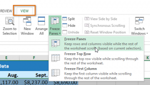
Next, on the ribbon click the View tab, then click the Window group and then Freeze Pane. Thiswill give you the options of,
Freeze Panes, which will freeze both the selected rows and columns together, or gives you the option of freezing more than one row or column.
Freeze Top Row will just freeze the top row.
Freeze First Column will just freeze the first column on the left.
To unfreeze the panes just go back on to the ribbon, to the Freeze pane panel and click Unfreeze Pane.