Get a callback from our team within 20 minutes during business hours.
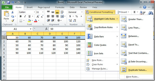
Sometimes when you are using Excel spreadsheets, you may find that you need to check cells for duplicate values, for example if you have merged data from two worksheets into one and you have to check if data has been duplicated. There are various ways of finding the duplicate values in content, but the simplest way to do this can be done using the Conditional Formatting button on the Home tab.
Select the columns and rows that you need to check for duplicates. You can click individual columns or rows, or you can hold down the Ctrl button and then select them. Then click on the Home tab and then the Conditional Formatting button to bring up the options box.
From the Conditional Formatting options box, click on the Highlight Cells Rules option and then select Duplicate Values.
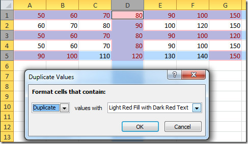
In the Duplicate Values dialogue box you can use the drop down menu to to choose how you want the duplicated values highlighted. Use the drop down menu to select the colour of the cell and the text and then click OK to finish.
Unique Values
You can also use the conditional formatting button to highlight Unique Values in a spreadsheet. Follow the same procedure as above then when you are in the Duplicate Values dialogue box, click on Unique in the drop down menu. This will now highlight the Unique Values in the spreadsheet.