The IF function in Excel can be very helpful for data analysis and conditional formatting. Below is an example of a way that the IF function can be used. The general formula for an IF function is: =IF(cell value, “value if true”, “value if false”) .
For a value “greater than” you use >
For a value “less than” you use <
For a value “greater or equal to” you use >=
For a value “less or equal” to you use <=
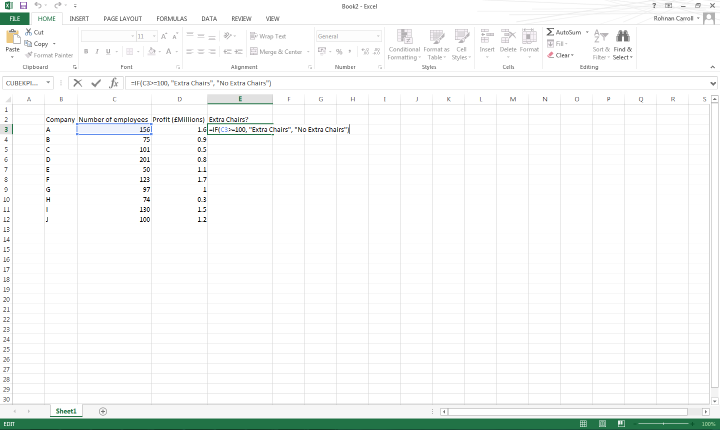
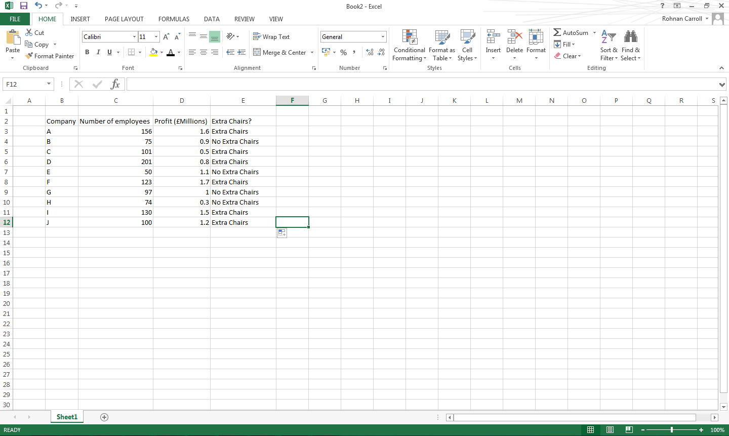
We have information about company A to J, we need to get extra chairs if the company has over 100 employees, this can be done using the IF function.
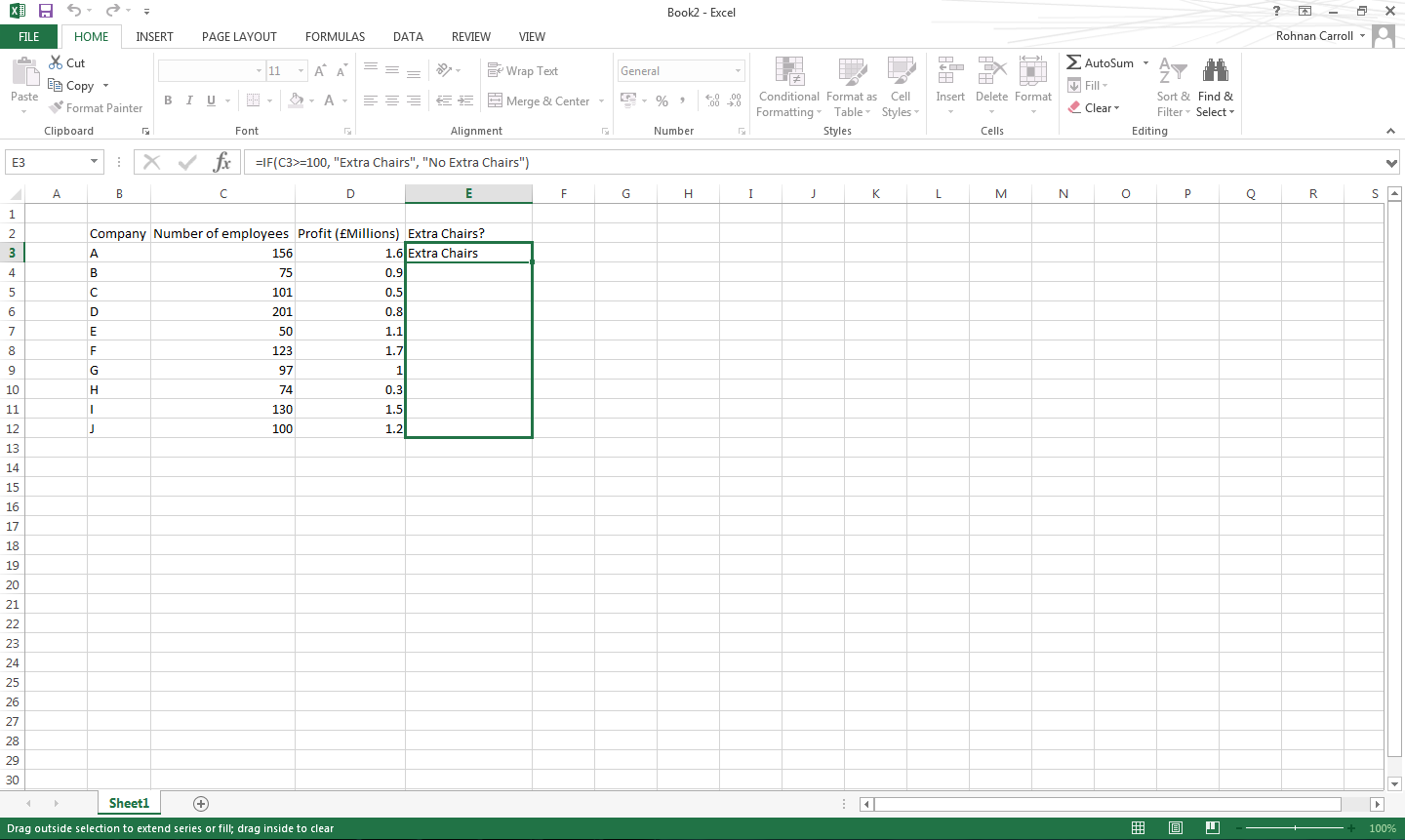
The formula used would be =IF(C3>=100, “Extra Chairs”, “No Extra Chairs”), you can then drag the formula down to all other cells you want to employ the formula in.
This will then populate the selected cells with either “Extra Chairs” if the value is 100 or over, or “No Extra Chairs” if the value is less than 100.
If you didn’t want to show anything if the value was false, so in this case “No Extra Chairs”, the formula would be =IF(C3>=100, “Extra Chairs”, “”).
If you wanted to do an IF formula based on two values, you use the IFAND function, the general formula for this is =IF(AND(cell value 1, call value 2) “value if true”, “value if false”).
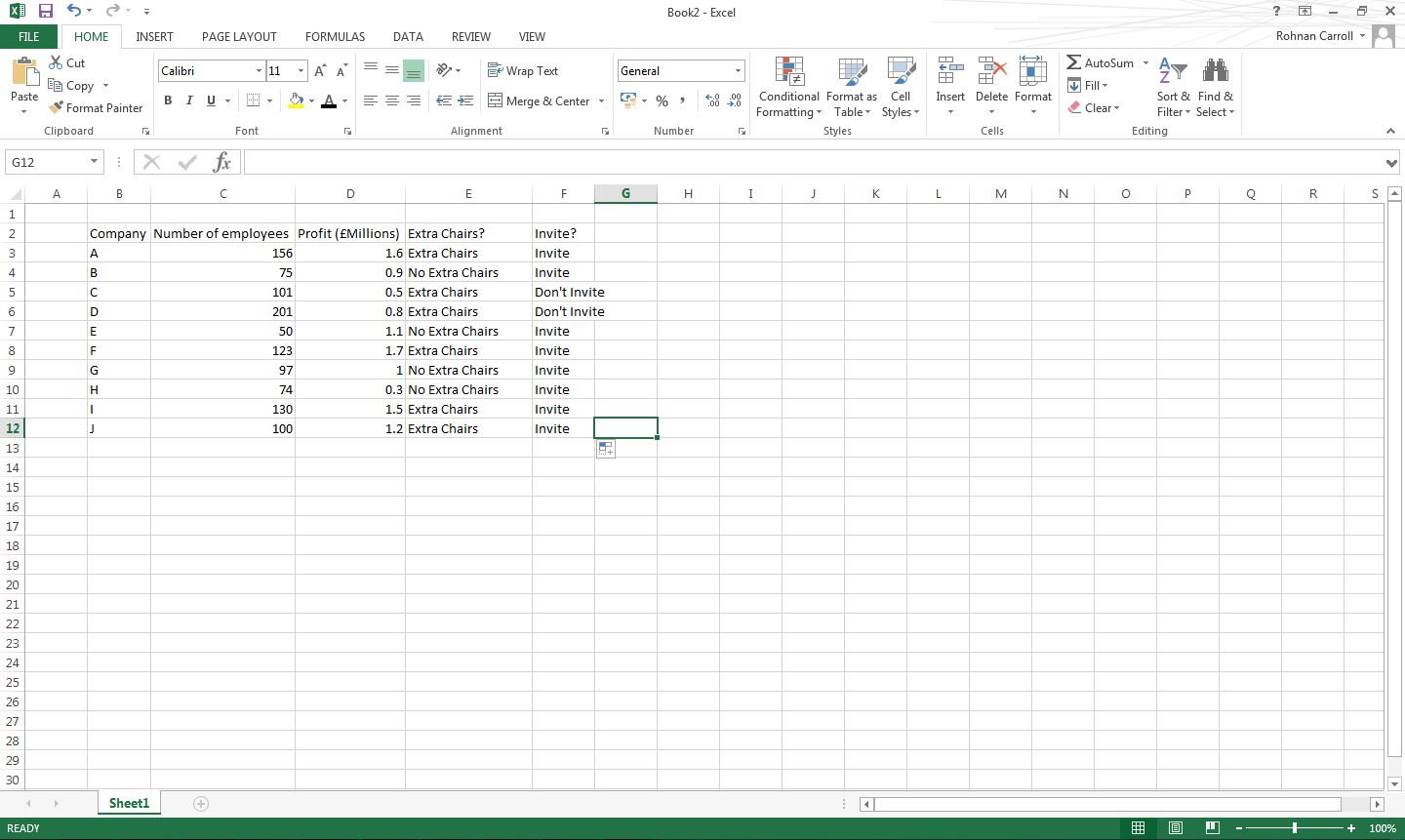
In the below example we want to show “Invite” if the company has 100 employees or more and their profits are over £1million. To do this you use the formula =IF(AND(C3>=100, D3<1), “Don’t Invite”, “Invite”). 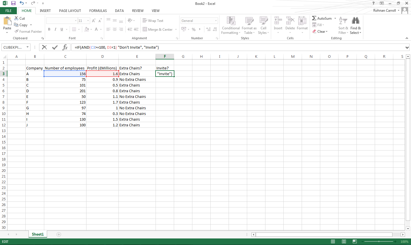
You can then apply the formula to every required cell as previously shown.